Lecture 04: Data Generating Processes and Statistical Models
Joseph Rudoler
2026-01-06
Recap: Sampling and Simulation
Last lecture we learned:
- How to sample from probability distributions
- IID sampling and sampling with/without replacement
- How to simulate complex random processes step by step
Today we formalize these ideas with data generating processes and statistical models.
Data Generating Processes
A key insight: all data is generated by some underlying process
- The process can be simple or complex
- Deterministic or stochastic
- Observed or unobserved
Thinking about data generating processes (DGPs) is fundamental to analyzing data.
Statistical Models
A statistical model is a formal mathematical representation of a DGP.
- Describes the probability distribution of the data
- Allows precise statements about generated data
- Tells us likelihood of certain values, expected values, etc.
Example: Coin Flips
DGP: Flipping a coin (heads or tails)
Statistical Model: Bernoulli distribution
\[P(X) = \begin{cases} p & \text{if } X = 1 ~\text{(heads)} \\ 1 - p & \text{if } X = 0 ~\text{(tails)} \end{cases}\]
For a fair coin: \(p = 0.5\)
Models are Reductive
The Bernoulli model ignores many factors:
- Weight of the coin
- Force of the flip
- Air resistance
But it accurately describes the outcomes — and that’s what matters!
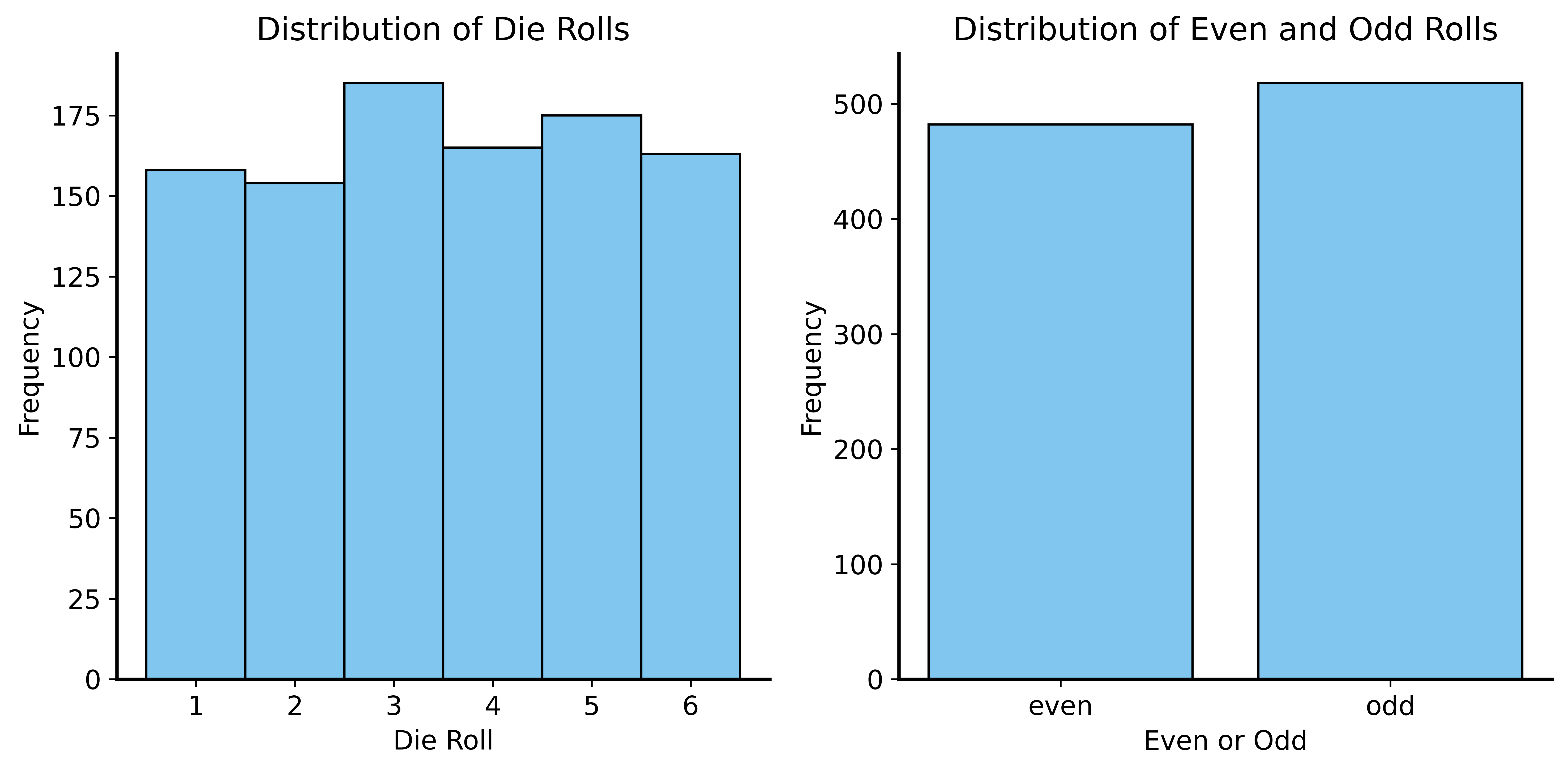
Example: Dice → Coin
Roll a die 100 times. Record whether each roll is even or odd.
- 3 even numbers (2, 4, 6)
- 3 odd numbers (1, 3, 5)
- Each outcome has probability 1/6
Result: P(even) = P(odd) = 0.5
This is statistically identical to flipping a fair coin!
Dice → Coin Visualization
The Goal of Statistical Modeling
Find a simple model that captures essential features of the DGP.
- We don’t always know the true DGP
- Often we don’t know anything about it!
- Approach: “guess and check”
- Start simple
- See how well it describes the data
- Try more complex models if needed
Challenges with Finite Samples
Hard to tell if you have a good model with limited data.
Extreme example: Flip a coin once
- Observed proportion of heads: 0 or 1
- Expected proportion: 0.5
- Impossible to observe the expected proportion!
You can’t learn much about tendencies from a single observation.
The Roommate Problem
Scenario: You and your roommate flip a coin to decide who takes out the trash.
- You always choose tails
- Best of 10 series
- Result: 3 heads, 7 tails
Your roommate: “That’s not fair! You rigged the coin!”
Is your roommate justified?
Distinguishing Models
| Scenario | P(3 heads in 10 flips) |
|---|---|
| Fair coin (p = 0.5) | ~11.7% |
| Biased coin (p = 0.25) | ~25.0% |
With 10 flips, you have some information but not enough to be confident.
Distinguishing Models (More Data)
| Scenario | P(30 heads in 100 flips) |
|---|---|
| Fair coin (p = 0.5) | ~0.002% |
| Biased coin (p = 0.25) | ~4.6% |
With more data, evidence becomes much stronger!
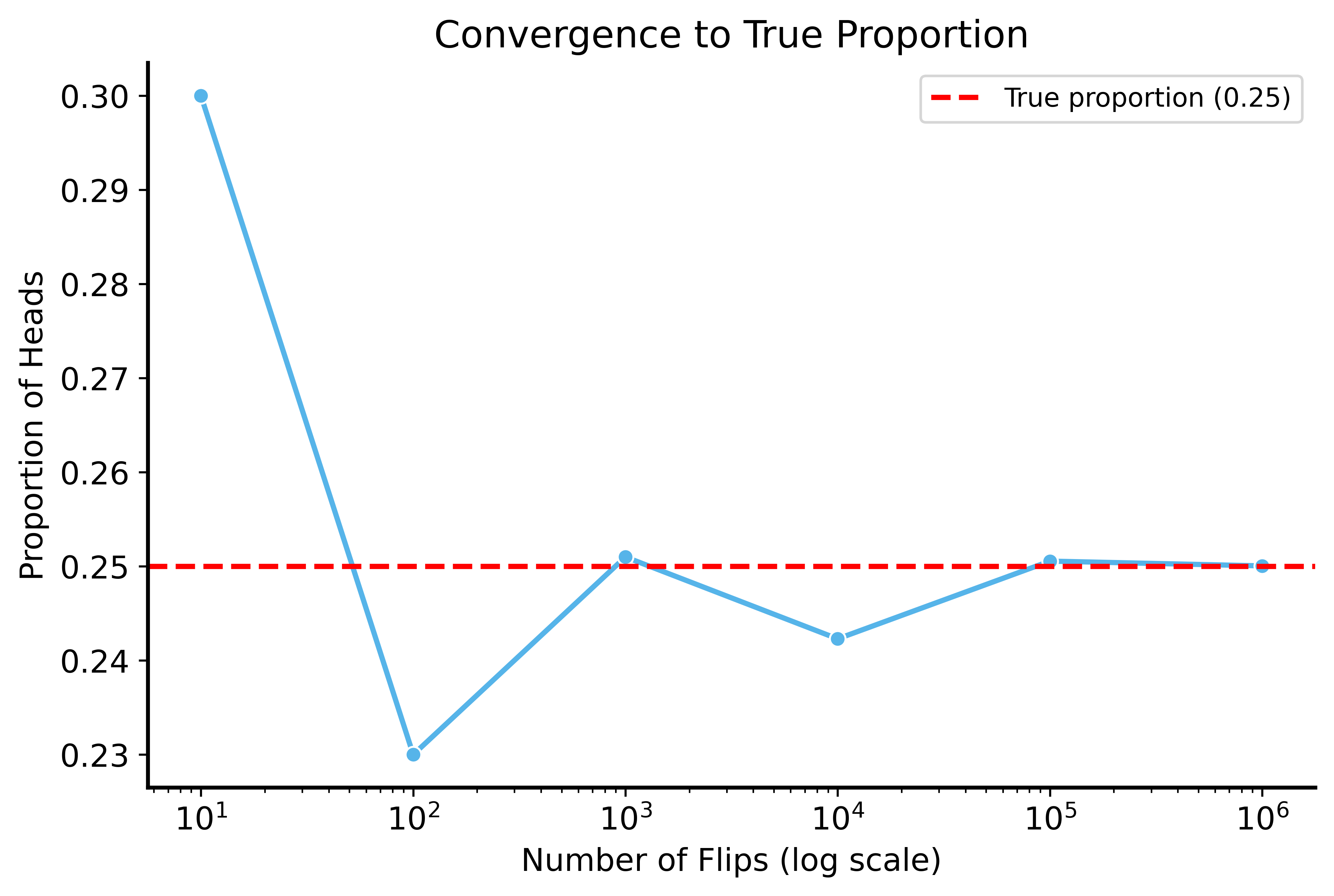
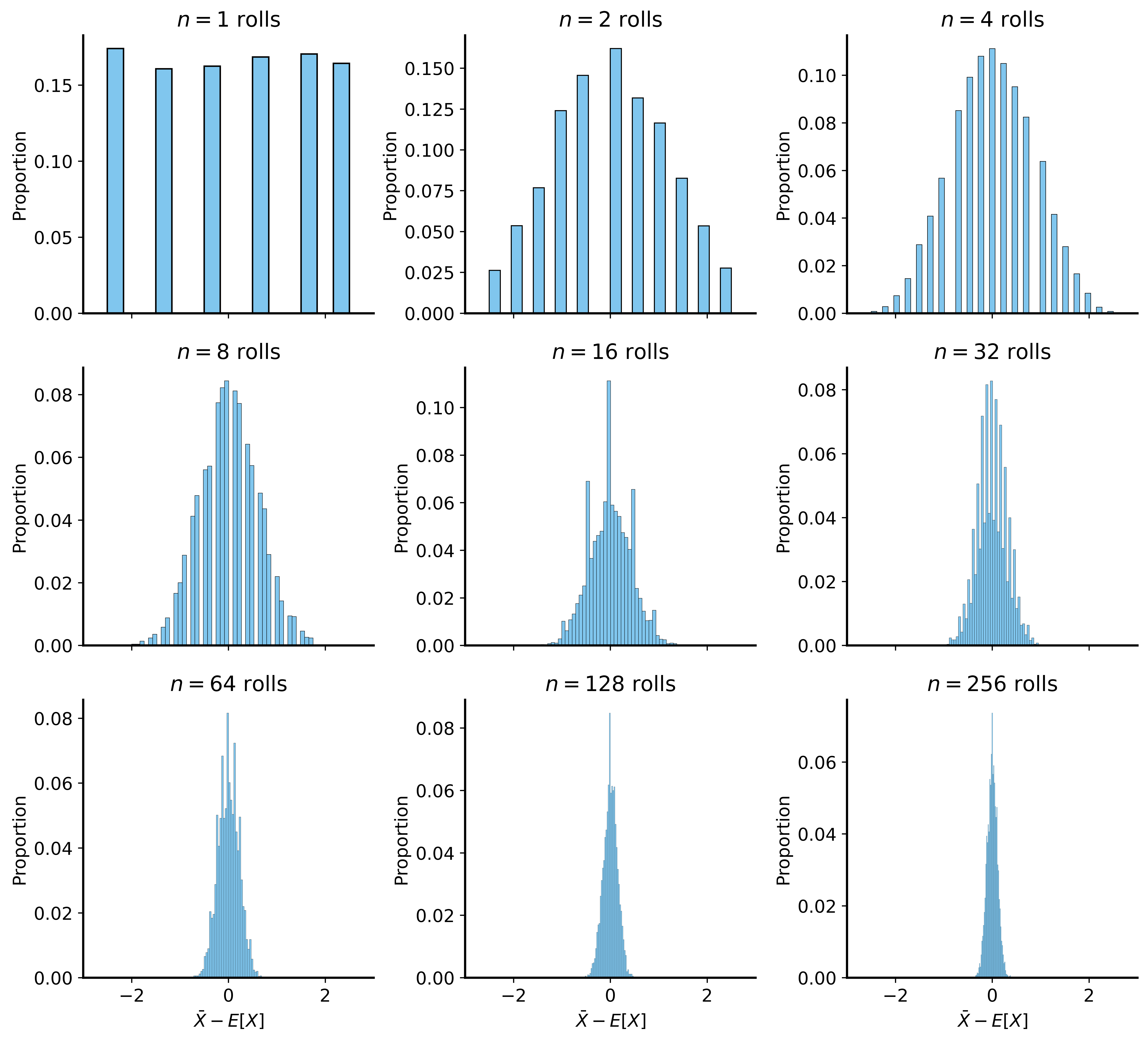
Law of Large Numbers
As sample size increases, the sample mean converges to the population mean.
Formally: Let \(X_1, X_2, \ldots, X_n\) be i.i.d. random variables with expected value \(\mathbb{E}[X]\)
\[\mathbb{P} \left[\lim_{n \to \infty} \bar{X}_n = \mathbb{E}[X]\right] = 1\]
The sample mean \(\bar{X}_n = \frac{1}{n} \sum_{i=1}^{n} X_i\) converges to the true mean.
LLN in Action
LLN: Multiple Simulations
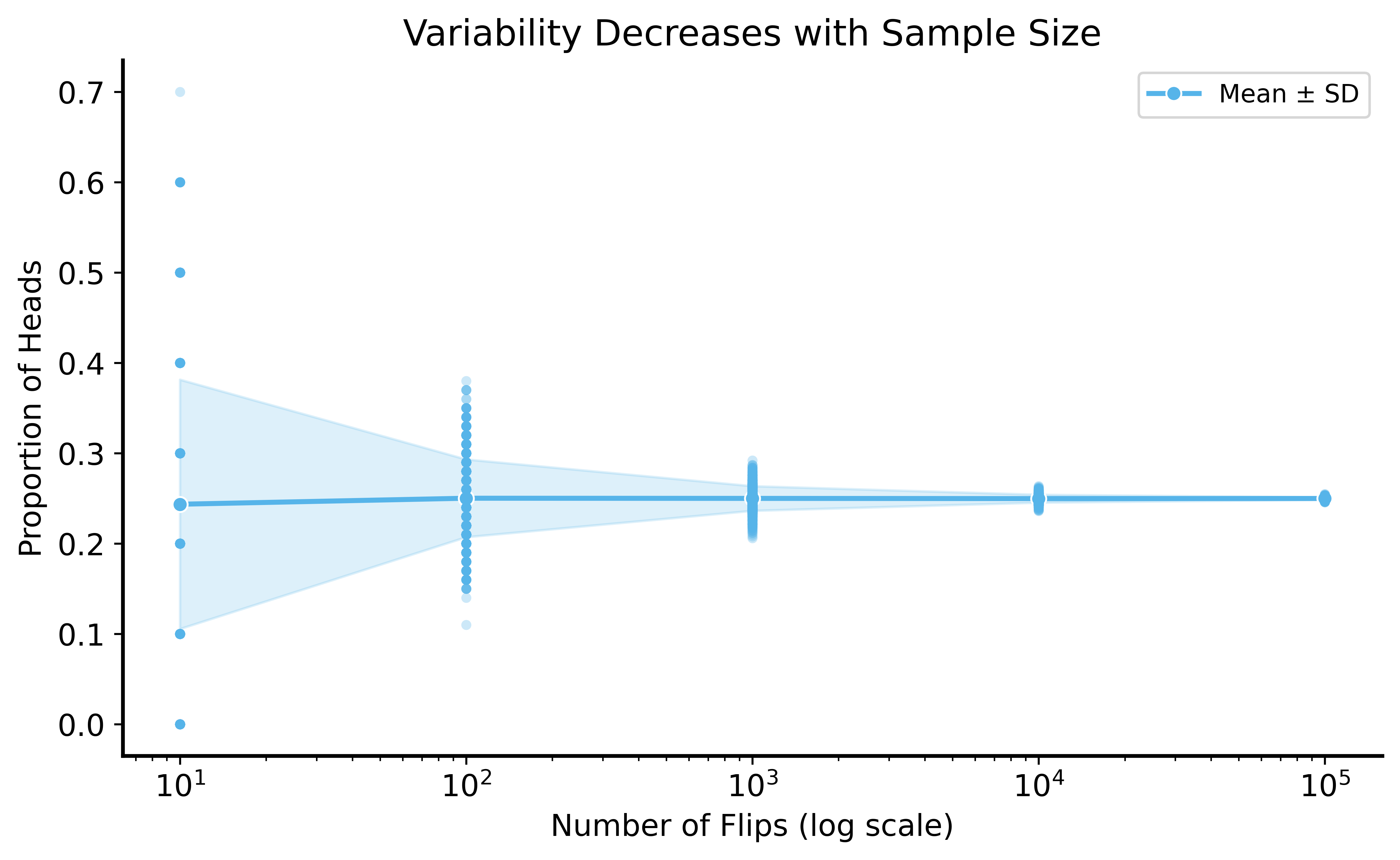
Key Insight from LLN
As sample size increases:
- Sample mean gets closer to true mean (on average)
- Variability decreases — estimates become more consistent
Practical implication: More data → more confident conclusions
Unbiased Estimators
Notice: even with high variability in small samples, the sample mean is centered around the true mean.
An estimator is unbiased if its expected value equals the true parameter.
\[\mathbb{E}[\bar{X}] = \mu\]
The LLN tells us that as \(n \to \infty\), the variance of the estimator decreases.
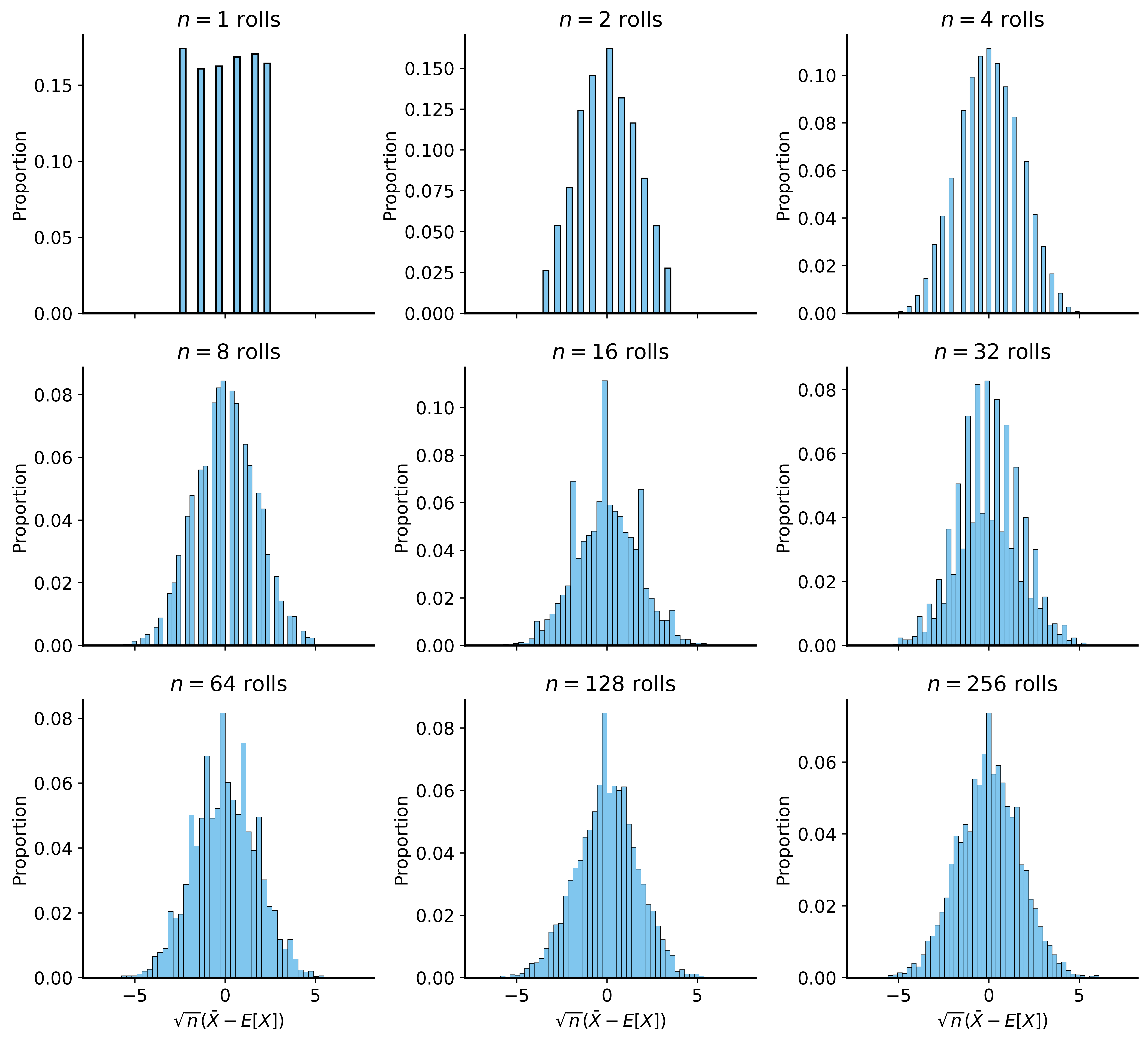
Central Limit Theorem
The sample mean converges to a normal distribution, regardless of the original distribution!
Formally: Let \(X_1, \ldots, X_n\) be i.i.d. with mean \(\mu\) and variance \(\sigma^2\)
\[\bar{X}_n \xrightarrow{d} N\left(\mu, \frac{\sigma^2}{n}\right)\]
Even if \(X\) is not normal, the average of many \(X\)’s is approximately normal!
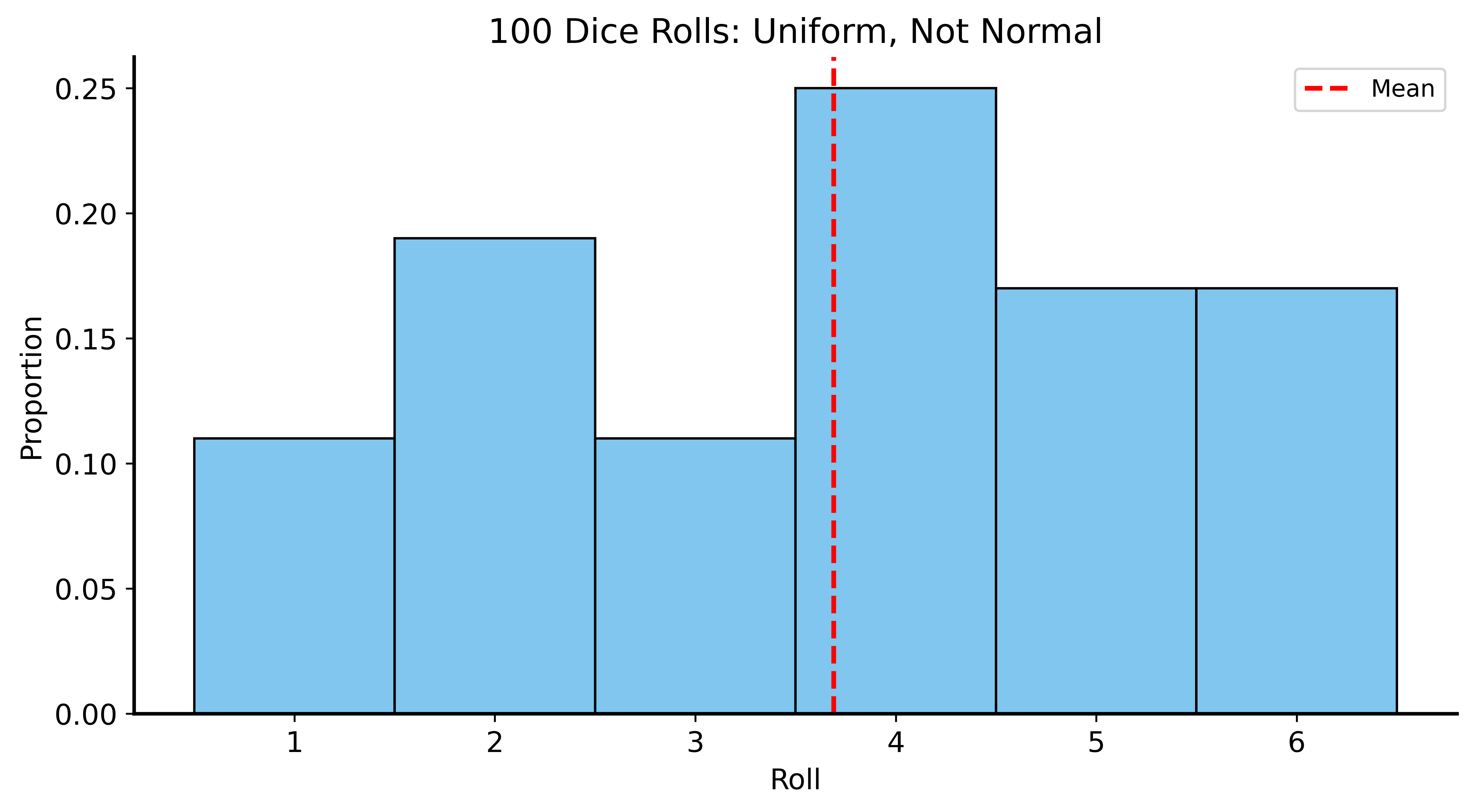
CLT Example: Dice Rolls
Rolling a die: uniform distribution from 1 to 6
- Expected value: \(E[X] = 3.5\)
- Clearly not normal
But what about the average of many dice rolls?
CLT Example: Single Die
CLT in Action
Why CLT Matters
Even when we don’t know the original distribution:
- We can use the normal distribution to model the sample mean
- This works for a huge class of DGPs
The normal distribution is:
- Symmetric
- Well-studied
- Easy to work with mathematically
Standard Errors
The CLT tells us the sample mean has variance \(\frac{\sigma^2}{n}\)
Standard error = standard deviation of the sample mean:
\[SE = \frac{\sigma}{\sqrt{n}}\]
As \(n\) increases, SE decreases → estimates become more precise
Standard Errors Visualized
Summary
Data Generating Processes
- All data comes from some underlying process
- Statistical models are simplified representations of DGPs
Law of Large Numbers
- Sample means converge to true means as \(n \to \infty\)
- More data → more confident conclusions
Central Limit Theorem
- Sample means are approximately normal (for large \(n\))
- Standard error decreases as \(\frac{1}{\sqrt{n}}\)
Next Time
Hypothesis Testing
- How to formally test claims about data
- Using sampling distributions to quantify uncertainty
- Making decisions under uncertainty