Lecture 05: Hypothesis Testing
Joseph Rudoler
2026-01-06
Recap
- All data comes from a data generating process (DGP)
- Statistical models describe the probability distribution of data
- LLN: Sample means converge to true means
- CLT: Sample means become normally distributed
Today: How to use these ideas to test claims about data
The Role of Inference
Drawing general conclusions (about a population) from specific observations (a sample)
Now that we have the building blocks, we can start making statistical inferences.
The Burden of Proof
How can we use statistics to “prove” something?
People often cite data as evidence:
- “Unemployment is lower than 4 years ago”
- “Player X has the highest scoring average”
These statements can sound iron-clad, but they often:
- Ignore complexity and uncertainty
- Cherry-pick supporting data
- Hide how data was collected/analyzed
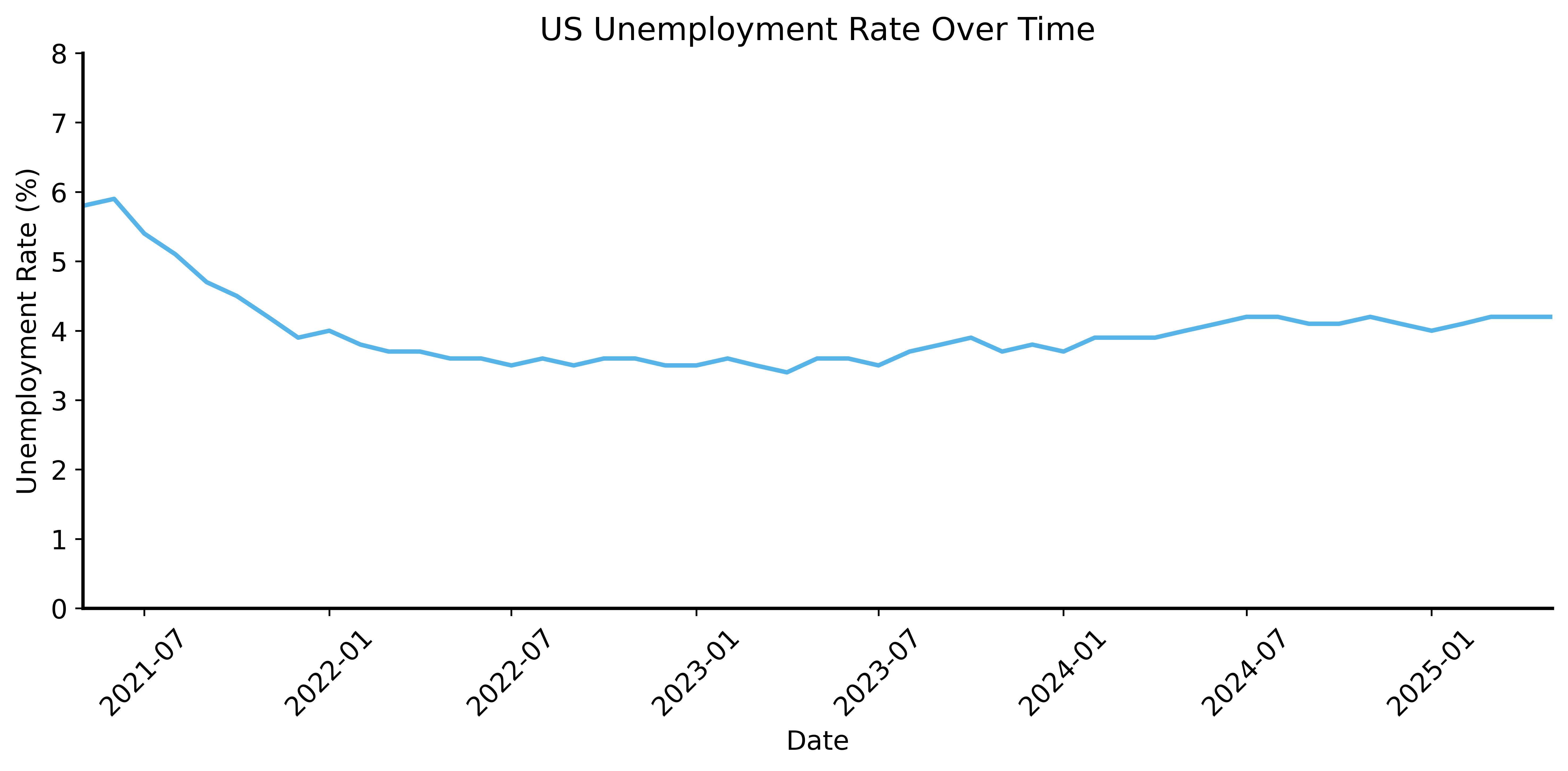
Example: Unemployment Data
A politician claims their policies reduced unemployment.
Evidence: “Unemployment rate is lower than 4 years ago”
Unemployment: Short View
Unemployment: The Bigger Picture
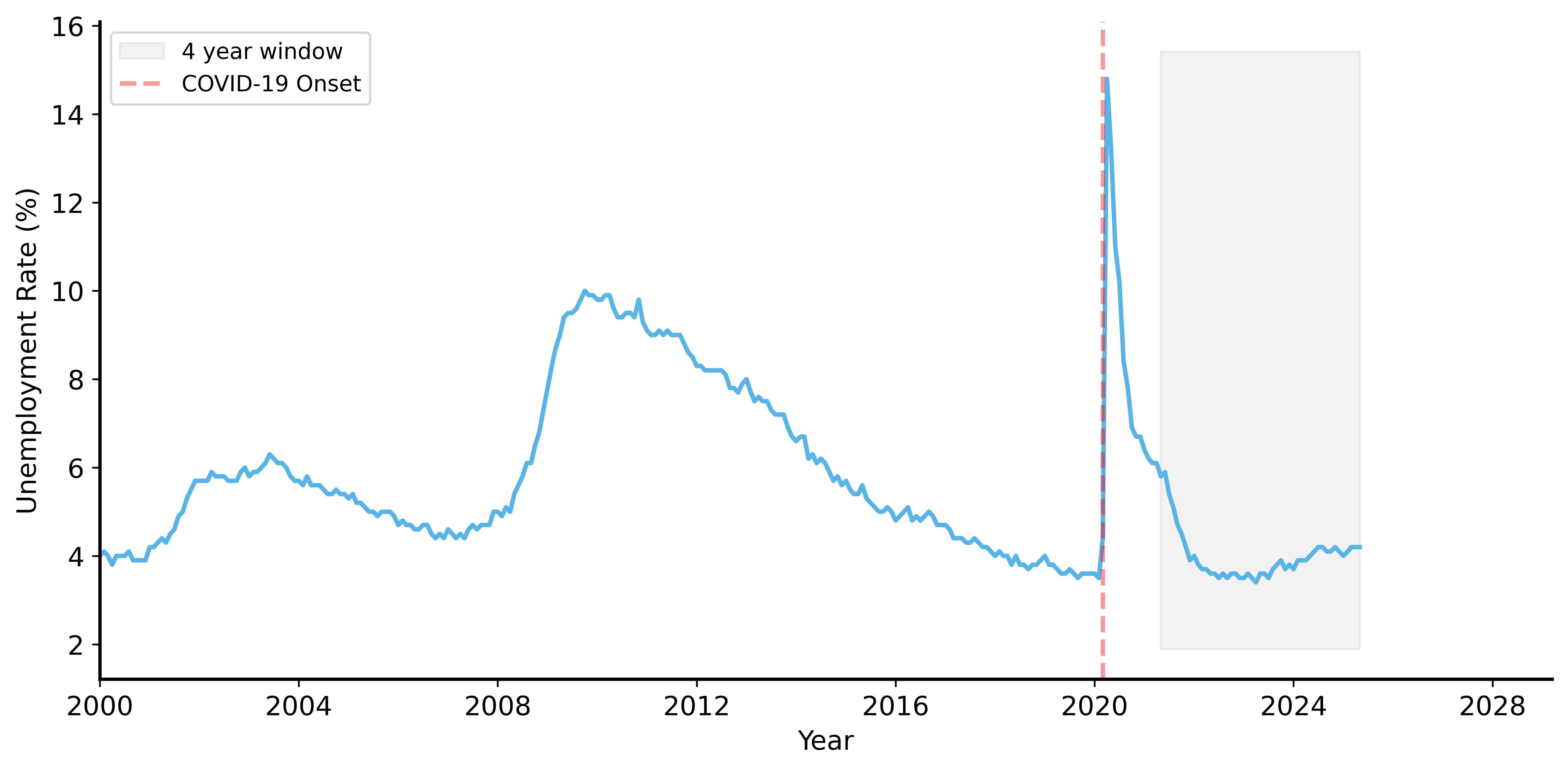
What the Data Really Shows
The politician’s claim is misleading:
- Unemployment spiked in 2020 (COVID-19 pandemic)
- By 2021, it wasn’t back to pre-pandemic levels
- The “decrease” is recovery, not policy success
Key lesson: Always be skeptical about data presented as evidence
Sources of Uncertainty
- Alternative explanations: External factors (pandemic) vs. claimed cause (policy)
- Sampling variability: Data is collected from samples, not whole populations
- Cherry-picking: Different time periods → different conclusions
How do we know if a change is real or just random fluctuation?
The Burden of Proof
The person making the claim must provide evidence.
In statistics, “beyond reasonable doubt” means:
- Alternative explanations are so unlikely
- A reasonable person would ignore them
- But this is always a subjective judgment!
Formalizing Hypotheses
Make claims specific and testable:
Null hypothesis (\(H_0\))
- The status quo or baseline assumption
- Often a statement of “no effect” or “no difference”
Alternative hypothesis (\(H_1\))
- The claim we want to test
- Logical complement of \(H_0\) (true when \(H_0\) is false)
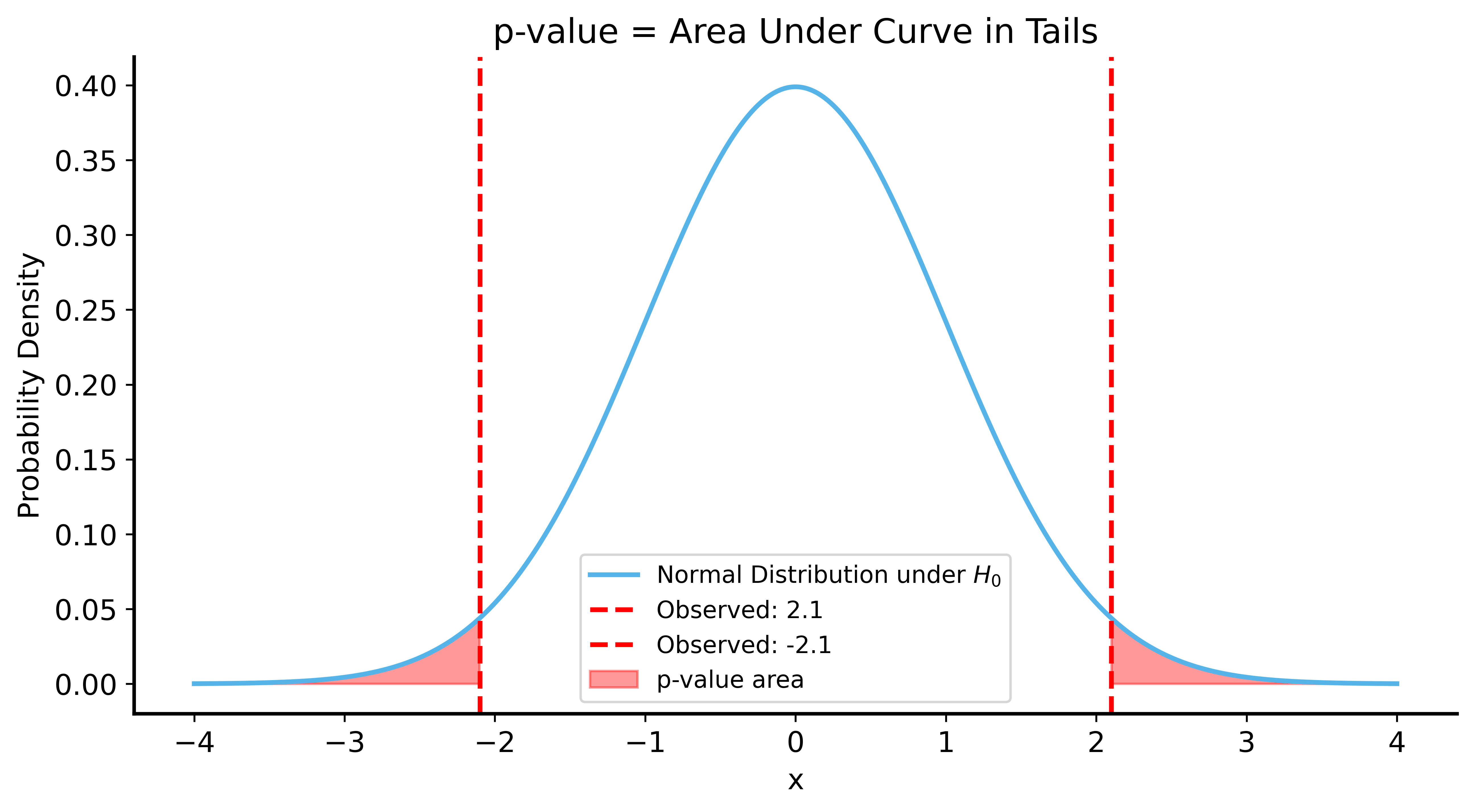
The p-value
Definition: The probability of observing data at least as extreme as what we observed, assuming \(H_0\) is true.
If \(p\) is very small:
- Data is unlikely under \(H_0\)
- We reject \(H_0\) in favor of \(H_1\)
Visualizing the p-value
Statistical Significance
The p-value is compared to a threshold \(\alpha\) (your risk tolerance)
- If \(p < \alpha\): result is statistically significant
- If \(p \geq \alpha\): result is not statistically significant
Common choice: \(\alpha = 0.05\) (5% chance of wrongly rejecting \(H_0\))
Better practice: Report the actual p-value, not just “significant” or “not”
Important Notes
- \(H_0\) and \(H_1\) must be mutually exclusive (one true → other false)
- \(H_0\) and \(H_1\) must be exhaustive (one must be true)
Hypothesis testing does NOT provide absolute certainty:
- Failing to reject \(H_0\) ≠ \(H_0\) is true
- Rejecting \(H_0\) ≠ \(H_1\) is definitely true
Worked Example: The Rigged Coin
Your roommate accuses you of using a rigged coin.
- You always choose tails
- Result: 3 heads, 7 tails in 10 flips
Can we test this claim?
Setting Up the Hypotheses
- \(H_0\) (null): The coin is fair (\(p \geq 0.5\))
- \(H_1\) (alternative): The coin is rigged toward tails (\(p < 0.5\))
This is a one-sided test — we only care if the coin favors tails.
Simulating the Null Distribution
Strategy: Simulate flipping a fair coin many times, see how often we get results as extreme as observed.
This gives us a sampling distribution under \(H_0\).
Simulation Code
Code
rng = np.random.default_rng(56)
n_sims = 10000
n_flips = 10
prob_heads = 0.5
proportions = []

for i in range(n_sims):
    flips = rng.binomial(n=n_flips, p=prob_heads)
    proportions.append(flips / n_flips)

proportions = np.array(proportions)
p_value = np.mean(proportions <= 0.3)  # proportion ≤ observed
print(f"p-value: {p_value:.4f}")
p-value: 0.1702Visualizing the Result
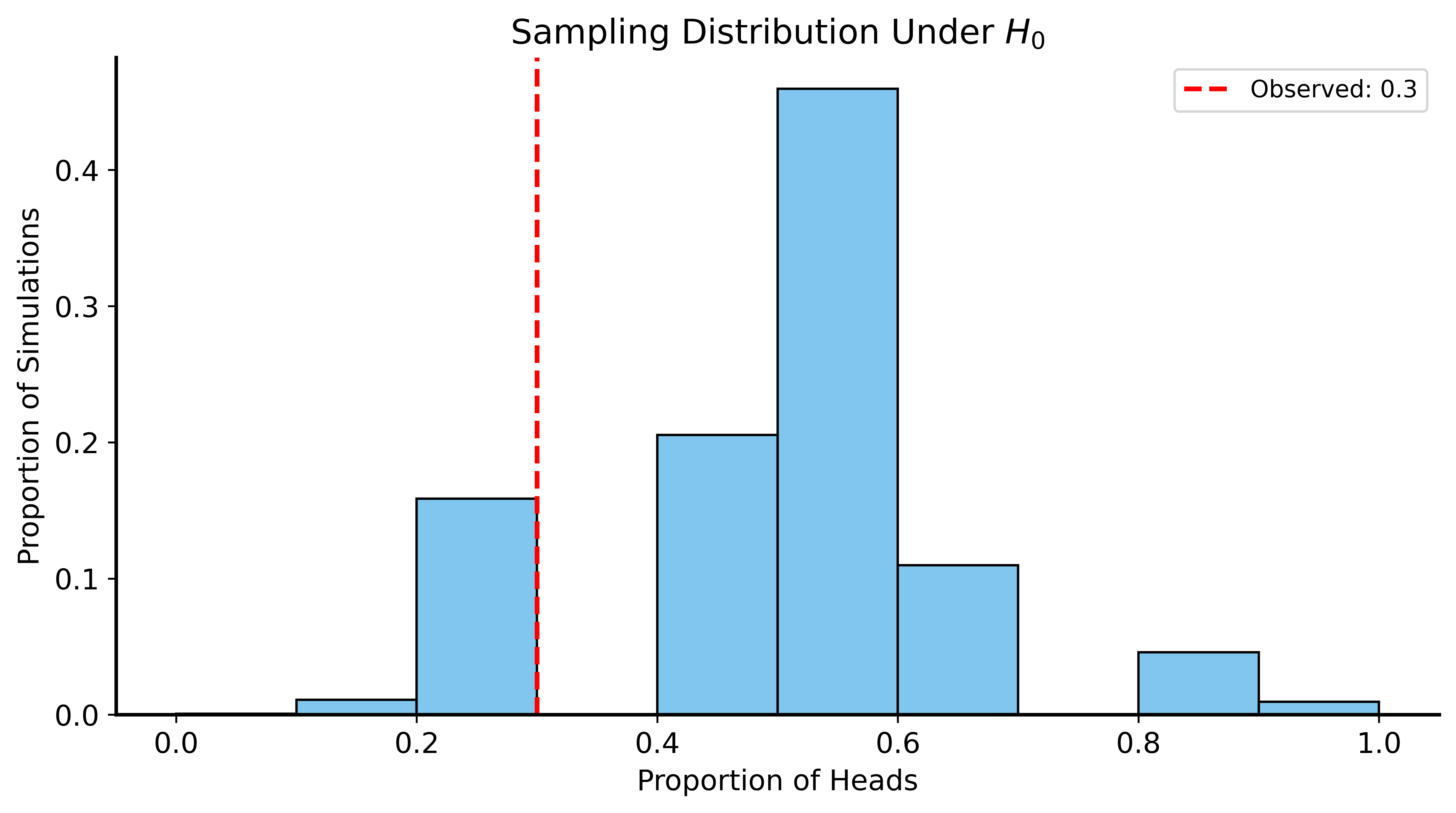
Conclusion
p-value ≈ 0.17 (17%)
Interpretation: Getting 3 heads in 10 flips happens ~17% of the time with a fair coin.
Verdict: Not enough evidence to support the roommate’s claim!
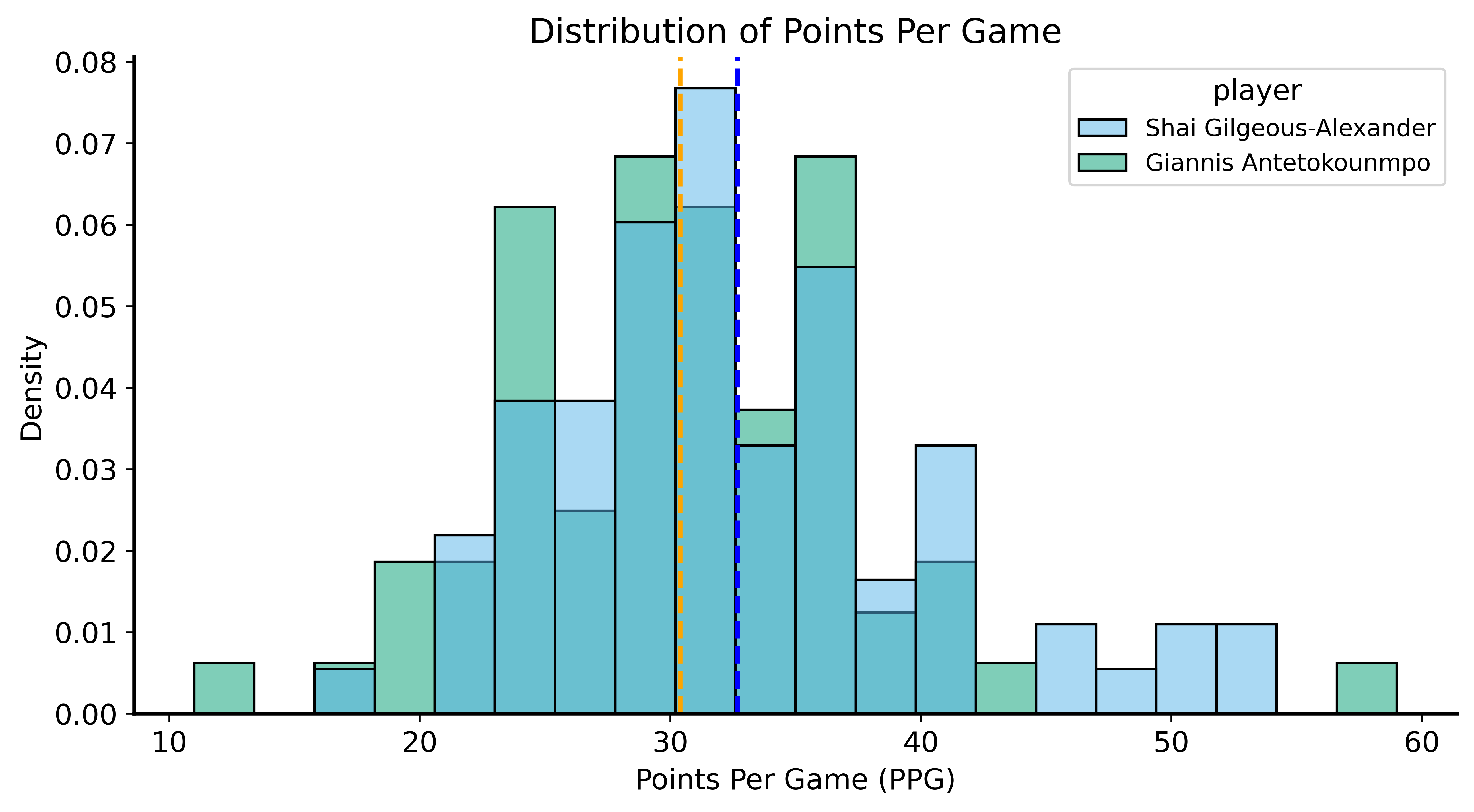
A More Complex Example: NBA MVP
“Shai Gilgeous-Alexander (SGA) is the best scorer in the NBA”
This is too vague to test! Let’s make it specific:
- Focus on points per game (PPG)
- Compare to next-best scorer (Giannis Antetokounmpo)
Formalizing the Hypothesis
Assumptions:
- Each player’s scoring follows a distribution with mean \(\mu\)
- By CLT, the average PPG is approximately normal
Hypotheses:
- \(H_0\): \(\mu_{\text{SGA}} \leq \mu_{\text{Giannis}}\)
- \(H_1\): \(\mu_{\text{SGA}} > \mu_{\text{Giannis}}\)
The Data
SGA: 32.68 PPG (SD: 7.54)
Giannis: 30.39 PPG
Scoring Distributions
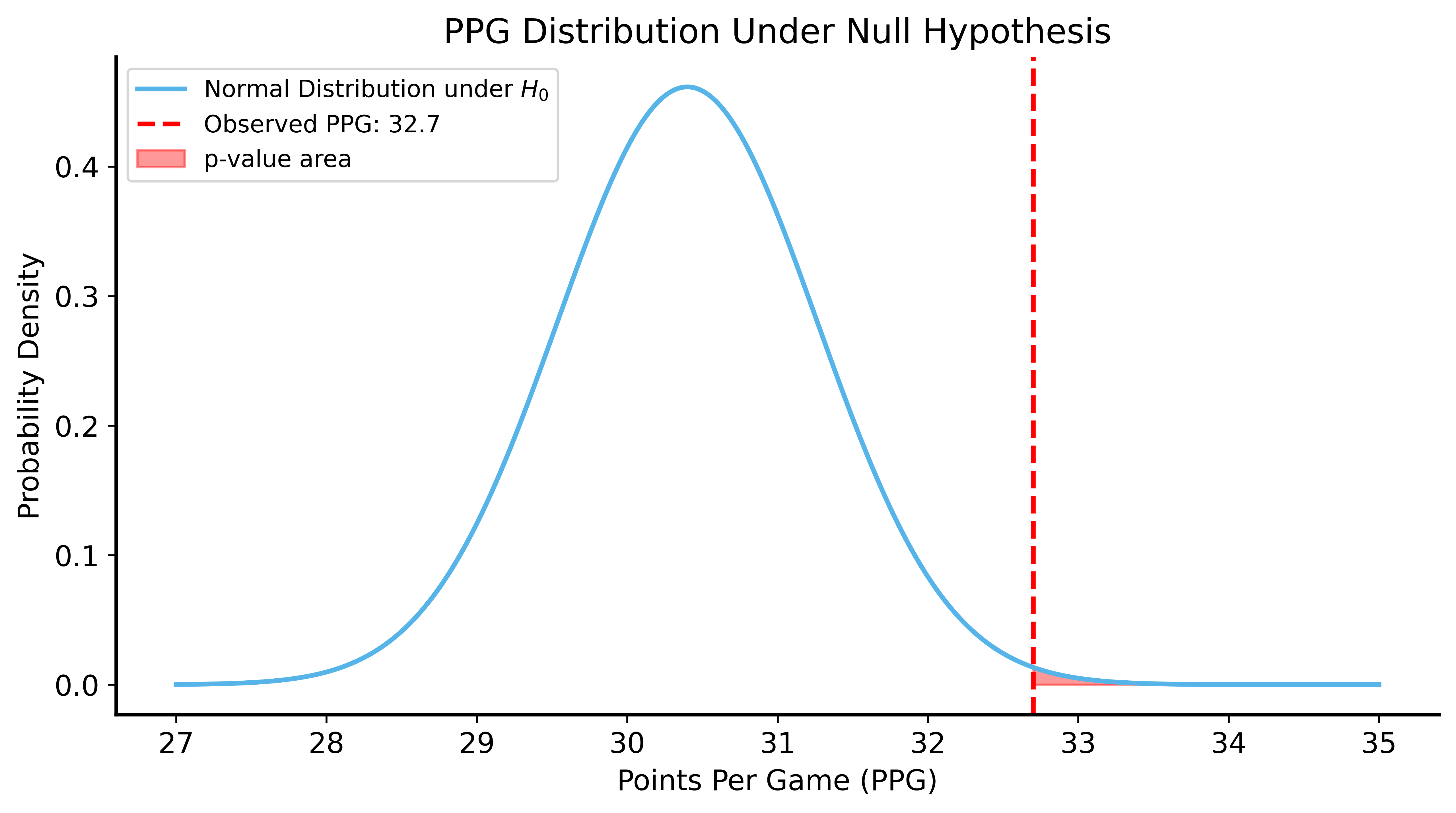
Using the CLT
Under \(H_0\): SGA’s true scoring rate = Giannis’s observed PPG (30.4)
Question: What’s the probability SGA scores ≥32.7 PPG if his true ability is 30.4?
p-value from CLT: 0.003910Visualizing the Null Distribution
Simulation Approach
We can also simulate without assuming normality!
Code
rng = np.random.default_rng(42)
n_sims = 5000
shai_simulated_ppg = []

for _ in range(n_sims):
    low_minus_high = np.sqrt(12 * shai_sample_std**2)
    simulated_scores = rng.uniform(low=30.4 - low_minus_high/2,
                                   high=30.4 + low_minus_high/2, size=76)
    simulated_ppg = np.mean(simulated_scores)
    shai_simulated_ppg.append(simulated_ppg)

p_value_simulated = np.mean(np.array(shai_simulated_ppg) >= 32.7)
print(f"p-value from simulation: {p_value_simulated:.4f}")
p-value from simulation: 0.0040Both Methods Agree!
- CLT p-value: ~0.004
- Simulation p-value: ~0.004
Conclusion: Very unlikely SGA would score 32.7 PPG if his true ability was only 30.4 PPG.
Errors in Hypothesis Testing
Two types of errors:
| Reject \(H_0\) | Don’t Reject \(H_0\) | |
|---|---|---|
| \(H_0\) true | Type I (false positive) | ✓ Correct |
| \(H_0\) false | ✓ Correct | Type II (false negative) |
- Type I error rate = \(\alpha\) (our significance threshold)
- Type II error rate = \(\beta\)
Summary
Hypothesis Testing Framework
- Define null and alternative hypotheses
- Collect data
- Compute test statistic
- Find p-value (probability of data under \(H_0\))
- Compare to significance threshold \(\alpha\)
Key Points
- p-values quantify evidence against \(H_0\)
- Simulation can generate sampling distributions
- Always report p-values, not just “significant/not”
Next Time
Confidence Intervals and Bootstrapping
- Quantifying uncertainty differently
- Resampling methods
- No assumptions about distributions needed!