Lecture 09: Regression Inference and Multiple Regression
2026-01-06
Recap: Linear Regression
\[Y = \beta_0 + \beta_1 X + \epsilon\]
- \(\beta_0\): intercept
- \(\beta_1\): slope
- \(\epsilon\): error term (random noise)
We use data to estimate \(\hat{\beta}_0\) and \(\hat{\beta}_1\)
Sampling Variability in Regression
Different samples → different estimates of \(\beta\)
This is the same sampling variability we’ve discussed throughout the course!
Hypothesis Testing in Regression
Common question: Is there a relationship between \(X\) and \(Y\)?
Hypotheses:
- \(H_0\): \(\beta_1 = 0\) (no relationship)
- \(H_1\): \(\beta_1 \neq 0\) (there is a relationship)
Simulating the Null Distribution
How can we generate \(\hat{\beta}_1\) values under \(H_0\)?
Permutation test: Shuffle \(Y\) values to break the \(X\)-\(Y\) relationship
Permutation Test for Regression
Code
def permutation_test_regression(data, x_col, y_col, n_permutations=1000, rng=None):
    if rng is None:
        rng = np.random.default_rng()

    # Observed slope
    model = smf.ols(f'{y_col} ~ {x_col}', data=data).fit()
    observed_beta = model.params[x_col]

    # Permutation distribution
    perm_betas = []
    for _ in range(n_permutations):
        y_perm = rng.permutation(data[y_col])
        perm_model = smf.ols(f'{y_col} ~ {x_col}',
                              data=data.assign(**{y_col: y_perm})).fit()
        perm_betas.append(perm_model.params[x_col])

    perm_betas = np.array(perm_betas)
    p_value = np.mean(np.abs(perm_betas) >= np.abs(observed_beta))

    return observed_beta, perm_betas, p_value
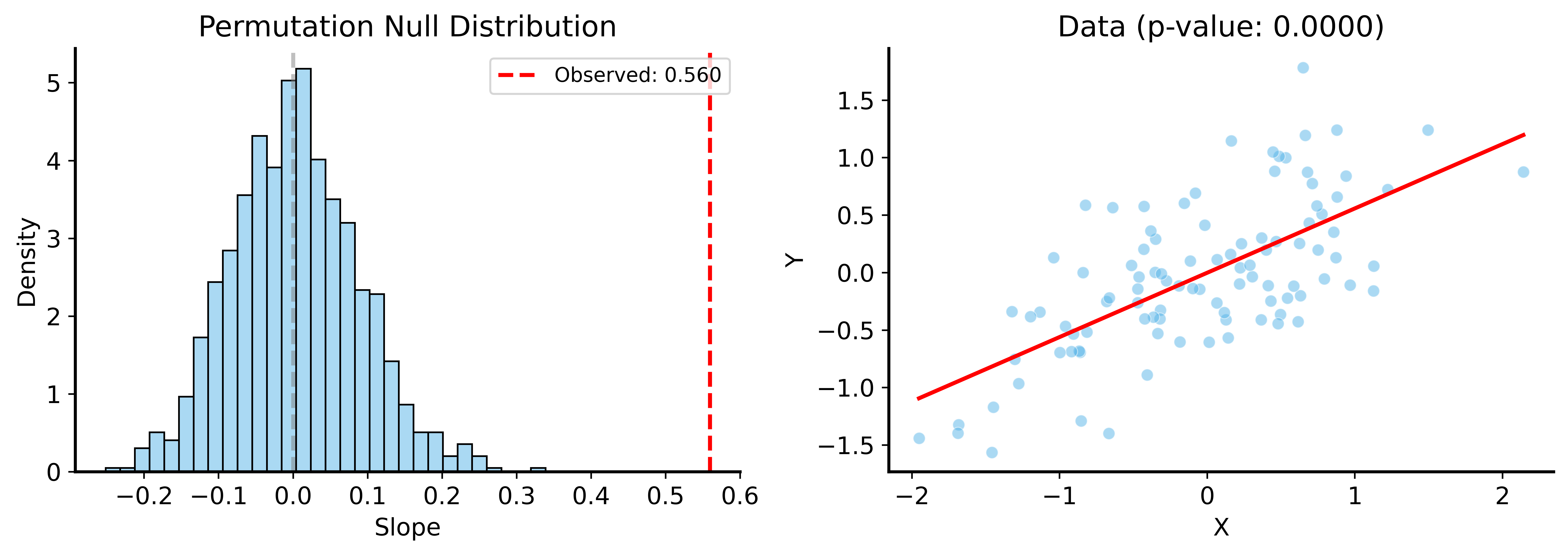
Example
Observed slope: 0.5596
Permutation p-value: 0.0000
Permutation vs Parametric
Parametric Results Match!
                            OLS Regression Results
==============================================================================
Dep. Variable:                      y   R-squared:                       0.443
Model:                            OLS   Adj. R-squared:                  0.437
No. Observations:                 100   F-statistic:                     77.87
Covariance Type:            nonrobust   Prob (F-statistic):           4.29e-14
==============================================================================
                 coef    std err          t      P>|t|      [0.025      0.975]
------------------------------------------------------------------------------
Intercept     -0.0023      0.049     -0.047      0.962      -0.100       0.095
x              0.5596      0.063      8.824      0.000       0.434       0.685
==============================================================================

Notes:
[1] Standard Errors assume that the covariance matrix of the errors is correctly specified.
Confidence Intervals for Regression
Use bootstrap to estimate CI for slope:
Code
def bootstrap_regression_ci(data, x_col, y_col, n_bootstraps=1000, alpha=0.05, rng=None):
    if rng is None:
        rng = np.random.default_rng()

    n = len(data)
    coefs = []
    for _ in range(n_bootstraps):
        sample = data.sample(n, replace=True)
        model = smf.ols(f"{y_col} ~ {x_col}", data=sample).fit()
        coefs.append(model.params[x_col])

    coefs = np.array(coefs)
    lower = np.percentile(coefs, 100 * alpha / 2)
    upper = np.percentile(coefs, 100 * (1 - alpha / 2))
    return coefs, lower, upper
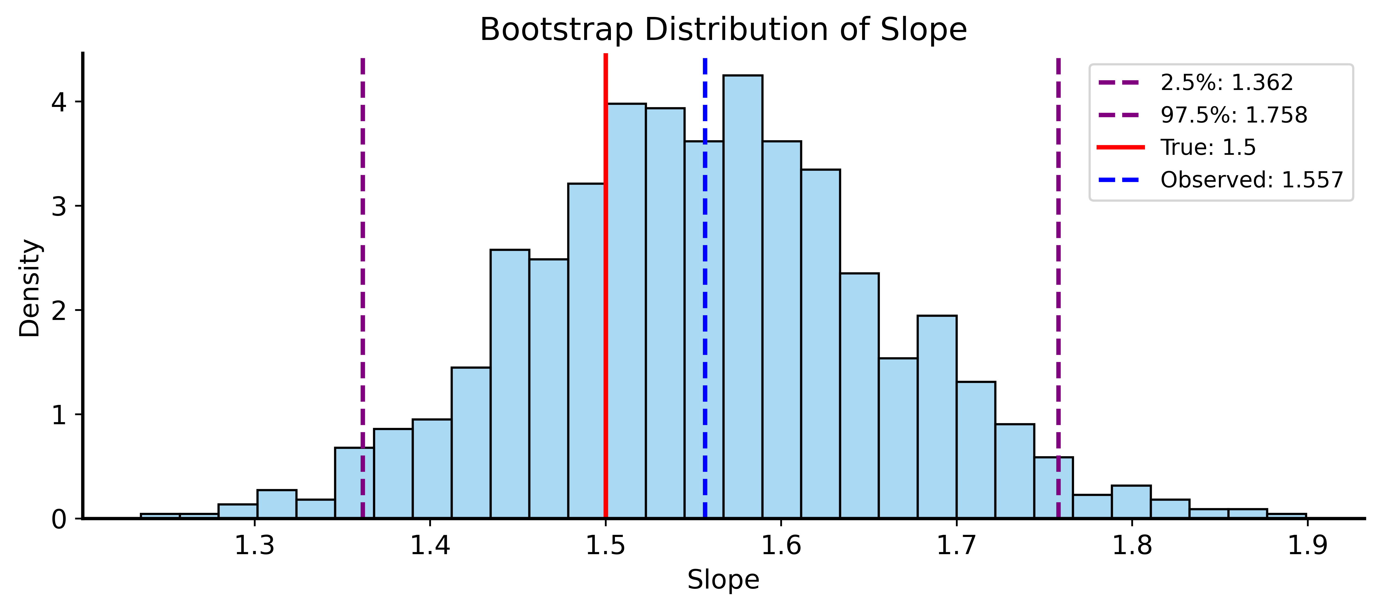
Bootstrap CI Example
Bootstrap 95% CI for slope: [1.362, 1.758]
True slope: 1.5

Parametric 95% CI: [1.352, 1.761]
Multiple Regression
What if we have multiple predictors?
\[Y = \beta_0 + \beta_1 X_1 + \beta_2 X_2 + \cdots + \beta_p X_p + \epsilon\]
This is multiple linear regression
The Data
| 0 |
4 |
4 |
2 |
6 |
| 1 |
1 |
1 |
2 |
6 |
| 2 |
1 |
1 |
2 |
10 |
| 3 |
4 |
2 |
3 |
15 |
| 4 |
3 |
3 |
2 |
10 |
Simple Regression: Father’s Education
                            OLS Regression Results
==============================================================================
Dep. Variable:                     G3   R-squared:                       0.023
Model:                            OLS   Adj. R-squared:                  0.021
No. Observations:                 395   F-statistic:                     9.352
Covariance Type:            nonrobust   Prob (F-statistic):            0.00238
==============================================================================
                 coef    std err          t      P>|t|      [0.025      0.975]
------------------------------------------------------------------------------
Intercept      8.7967      0.576     15.264      0.000       7.664       9.930
Fedu           0.6419      0.210      3.058      0.002       0.229       1.055
==============================================================================

Notes:
[1] Standard Errors assume that the covariance matrix of the errors is correctly specified.
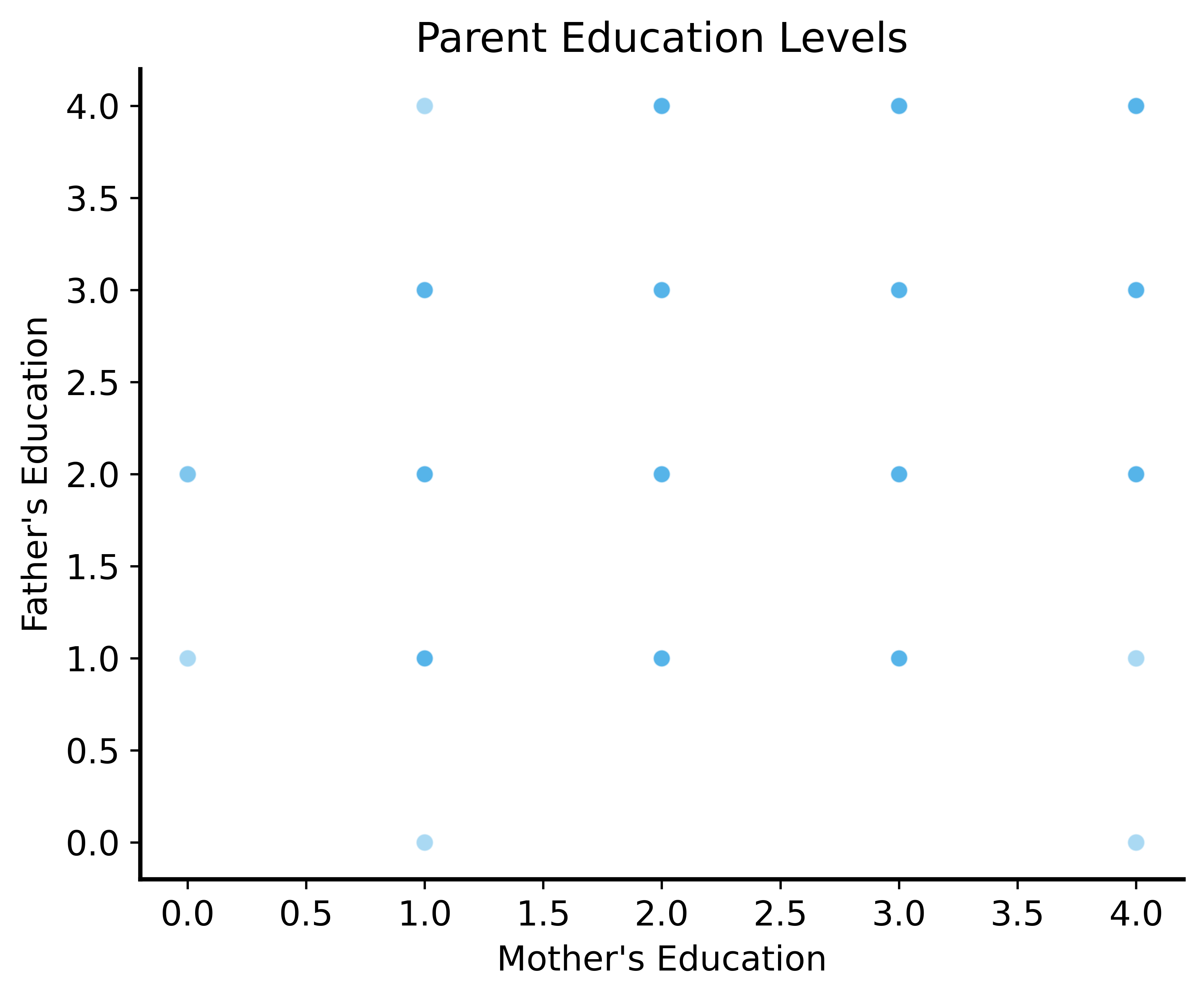
But Wait…
What about mother’s education?
Let’s look at how these variables relate:
| Fedu |
1.000 |
0.623 |
0.152 |
| Medu |
0.623 |
1.000 |
0.217 |
| G3 |
0.152 |
0.217 |
1.000 |
The Problem: Multicollinearity
Father’s and mother’s education are correlated!
- Students with educated fathers often have educated mothers
- Hard to separate individual effects
Multiple Regression to the Rescue
Include both predictors:
                            OLS Regression Results
==============================================================================
Dep. Variable:                     G3   R-squared:                       0.048
Model:                            OLS   Adj. R-squared:                  0.043
No. Observations:                 395   F-statistic:                     9.802
Covariance Type:            nonrobust   Prob (F-statistic):           7.01e-05
==============================================================================
                 coef    std err          t      P>|t|      [0.025      0.975]
------------------------------------------------------------------------------
Intercept      7.8205      0.648     12.073      0.000       6.547       9.094
Fedu           0.1176      0.265      0.443      0.658      -0.404       0.639
Medu           0.8359      0.264      3.168      0.002       0.317       1.355
==============================================================================

Notes:
[1] Standard Errors assume that the covariance matrix of the errors is correctly specified.
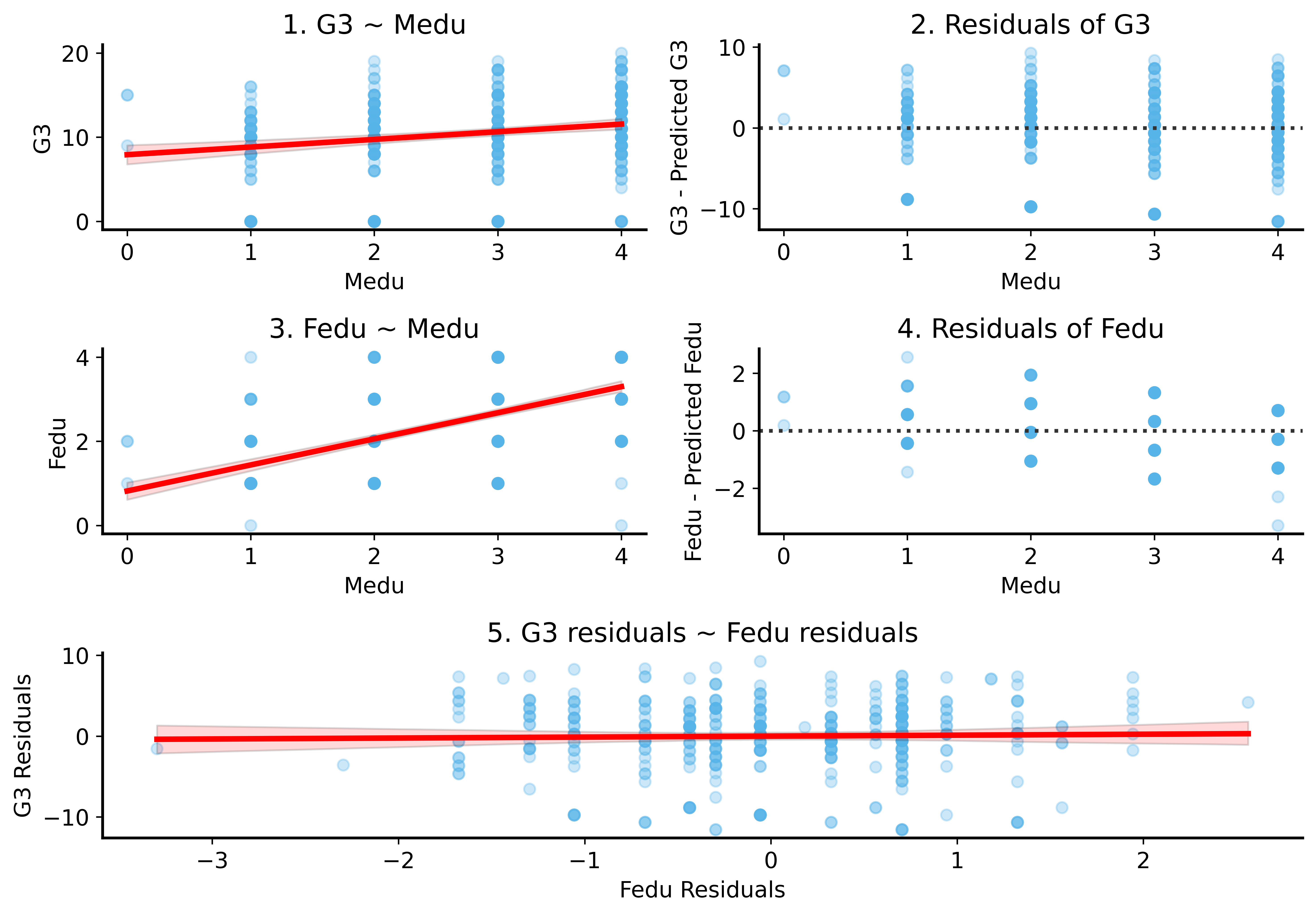
Interpretation
Before (Fedu only): significant effect
After (Fedu + Medu): Fedu effect shrinks, Medu dominates
Multiple regression controls for other variables!
Confounding Example
Does mother’s education cause better grades?
Or do they share a common cause (e.g., family wealth)?
- Wealth → can afford education for mom
- Wealth → can afford tutoring for student
The “Reverse” Regression
What if we regress Medu on G3?
                            OLS Regression Results
==============================================================================
Dep. Variable:                   Medu   R-squared:                       0.404
Model:                            OLS   Adj. R-squared:                  0.401
No. Observations:                 395   F-statistic:                     132.8
Covariance Type:            nonrobust   Prob (F-statistic):           9.00e-45
==============================================================================
                 coef    std err          t      P>|t|      [0.025      0.975]
------------------------------------------------------------------------------
Intercept      0.9051      0.136      6.658      0.000       0.638       1.172
Fedu           0.6080      0.040     15.319      0.000       0.530       0.686
G3             0.0299      0.009      3.168      0.002       0.011       0.048
==============================================================================

Notes:
[1] Standard Errors assume that the covariance matrix of the errors is correctly specified.
This suggests G3 “causes” Medu — obviously wrong!
Summary
Regression Inference
- Use permutation tests or bootstrap for hypothesis testing
- Same principles as before, applied to regression
Multiple Regression
- Include multiple predictors simultaneously
- Controls for confounding between predictors
Causality
- Regression shows association, not causation
- Need additional assumptions or experimental design