So begins “Understanding Uncertainty”, a course in statistical thinking and data science.
This is lecture 0. See the syllabus for an overview of the course.
Our basic goals for the course are:
to build a strong intuition about data, where it comes from, and what questions it can answer.
to learn the basic computational skills needed to manipulate and analyze data. Working with data also helps with (1)!
Why statistics?
Statistics is, essentially, the study of data and how to use it. People argue about the purpose of statistics, but basically you can do 3 things with data: (1) description, (2) inference, and (3) prediction.
Description
Descriptive statistics is the process of summarizing data. This can be done with numbers (e.g., mean, median, standard deviation) or with visualizations (e.g., histograms, boxplots). Descriptive statistics, importantly, are completely limited to the sample of data at hand.
Let’s load in some data and take a look at it.
The dataset contains Airbnb listings in New York City, including prices, locations, and other features.
Code
# from https://www.kaggle.com/datasets/arianazmoudeh/airbnbopendata# import the data on Airbnb listings in the New York Cityairbnb = pd.read_csv("../data/airbnb.csv")# data cleaningairbnb = airbnb.rename(columns={"neighbourhood_group": "borough"})airbnb = airbnb.dropna(subset=["borough", "price", "long", "lat"])airbnb["borough"] = airbnb["borough"].str.lower()airbnb["borough"] = airbnb["borough"].str.replace("manhatan", "manhattan")airbnb["borough"] = airbnb["borough"].str.replace("brookln", "brooklyn")# format the price columnairbnb['price'] = airbnb['price'].replace({'\\$': '', ',': ''}, regex=True).astype(float)# print the first 5 rowsairbnb[:5]
id
name
host_id
host_identity_verified
host_name
borough
neighbourhood
lat
long
country
...
service_fee
minimum_nights
number_of_reviews
last_review
reviews_per_month
review_rate_number
calculated_host_listings_count
availability_365
house_rules
license
0
1001254
Clean & quiet apt home by the park
80014485718
unconfirmed
Madaline
brooklyn
Kensington
40.64749
-73.97237
United States
...
$193
10.0
9.0
10/19/2021
0.21
4.0
6.0
286.0
Clean up and treat the home the way you'd like...
NaN
1
1002102
Skylit Midtown Castle
52335172823
verified
Jenna
manhattan
Midtown
40.75362
-73.98377
United States
...
$28
30.0
45.0
5/21/2022
0.38
4.0
2.0
228.0
Pet friendly but please confirm with me if the...
NaN
2
1002403
THE VILLAGE OF HARLEM....NEW YORK !
78829239556
NaN
Elise
manhattan
Harlem
40.80902
-73.94190
United States
...
$124
3.0
0.0
NaN
NaN
5.0
1.0
352.0
I encourage you to use my kitchen, cooking and...
NaN
3
1002755
NaN
85098326012
unconfirmed
Garry
brooklyn
Clinton Hill
40.68514
-73.95976
United States
...
$74
30.0
270.0
7/5/2019
4.64
4.0
1.0
322.0
NaN
NaN
4
1003689
Entire Apt: Spacious Studio/Loft by central park
92037596077
verified
Lyndon
manhattan
East Harlem
40.79851
-73.94399
United States
...
$41
10.0
9.0
11/19/2018
0.10
3.0
1.0
289.0
Please no smoking in the house, porch or on th...
NaN
5 rows × 26 columns
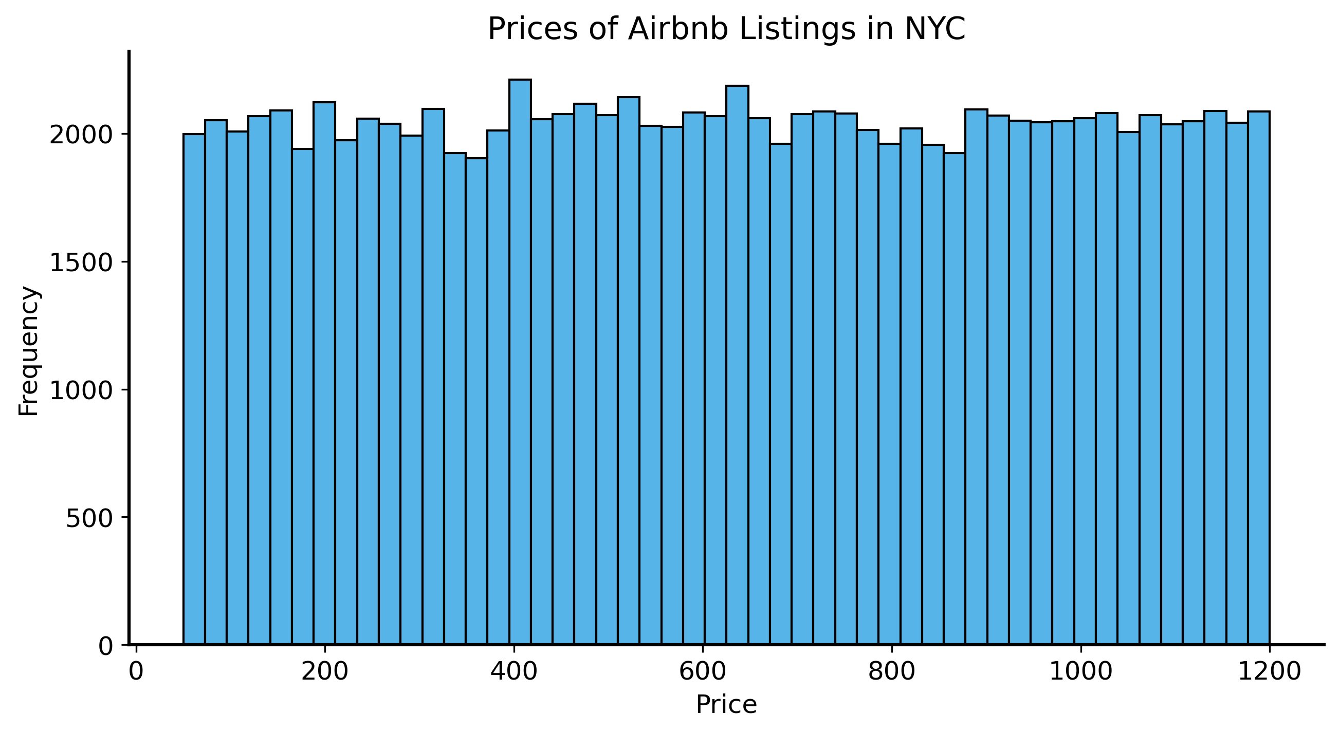
Now there’s a lot you can do, but let’s start by visualizing the prices of listings.
Code
# plot a histogram of the price columnplt.figure(figsize=(10, 5))plt.hist(airbnb['price'], bins=50)plt.title('Prices of Airbnb Listings in NYC')plt.xlabel('Price')plt.ylabel('Frequency')plt.show()
Computing statistics like the mean (average), standard deviation (average distance from the mean), and quartiles (top 25% and bottom 25%) is easy.
Code
airbnb["price"].describe()
count    102316.000000
mean        625.291665
std         331.677344
min          50.000000
25%         340.000000
50%         624.000000
75%         913.000000
max        1200.000000
Name: price, dtype: float64
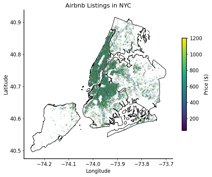
We can even use specialized libraries to make use of the geographic information in the data. For example, we can use the geopandas library to plot the locations of listings on a map of New York City.
Code
import geopandas as gpdfrom geodatasets import get_path# load the shapefile of NYC neighborhoodsnyc_neighborhoods = gpd.read_file(get_path('nybb'))nyc_neighborhoods = nyc_neighborhoods.to_crs(epsg=4326) # convert to WGS84# plot the neighborhoods with airbnb listingsnyc_neighborhoods.plot(figsize=(8, 8), color='white', edgecolor='black')# plot the airbnb listings on top of the neighborhoods# use the 'long' and 'lat' columns to create a GeoDataFrameairbnb_gdf = gpd.GeoDataFrame(airbnb, geometry=gpd.points_from_xy(airbnb['long'], airbnb['lat']), crs='EPSG:4326')# set the coordinate reference system to WGS84airbnb_gdf.plot(ax=plt.gca(), column="price", markersize=3, alpha=0.05, legend=True, cmap='viridis', legend_kwds={'shrink': 0.5, 'label': 'Price ($)'})plt.title('Airbnb Listings in NYC')plt.xlabel('Longitude')plt.ylabel('Latitude')plt.show()
There is a lot of information in the data, and we can summarize it in many different ways. But descriptive statistics only describe the data.
Why is this limiting? After all, we like data – it tells us things about the world and it’s objective and quantifiable.
The problem is that data is not always complete. In fact, it almost never is. And incomplete data can lead to misleading conclusions.
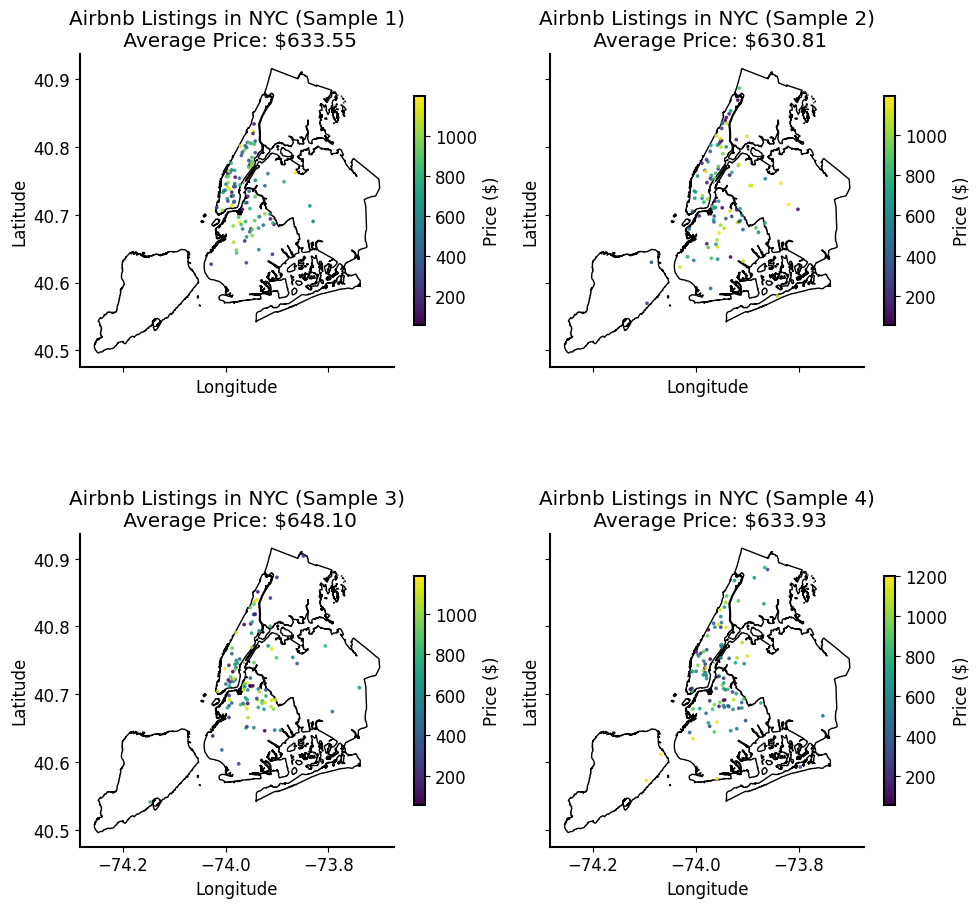
Let’s look at our Airbnb data again. What if instead of looking at the entire dataset, we only looked at a small “sample” or subset of the data?
Code
# separately plot 3 samples of airbnb listingsfig, ax = plt.subplots(2, 2, figsize=(10, 10), sharex=True, sharey=True)ax = ax.flatten()for i inrange(4):# sample 1000 listings sample = airbnb.sample(100, random_state=i)# plot the neighborhoods with airbnb listings nyc_neighborhoods.plot(ax=ax[i], color='white', edgecolor='black')# plot the airbnb listings on top of the neighborhoods# use the 'long' and 'lat' columns to create a GeoDataFrame airbnb_gdf_sample = gpd.GeoDataFrame(sample, geometry=gpd.points_from_xy(sample['long'], sample['lat']), crs='EPSG:4326')# set the coordinate reference system to WGS84 airbnb_gdf_sample.plot(ax=ax[i], column="price", markersize=3, alpha=0.8, legend=True, cmap='viridis', legend_kwds={'shrink': 0.5, 'label': 'Price ($)'}) ax[i].set_title(f'Airbnb Listings in NYC (Sample {i+1})\n Average Price: ${sample["price"].mean():.2f}') ax[i].set_xlabel('Longitude') ax[i].set_ylabel('Latitude')plt.tight_layout()plt.show()
Notice how the samples differ from one another. They have different geography and different prices. This means you can’t just look at the descriptive statistics of a single sample and draw conclusions about the entire population.
Sample vs. Population
A population is the entire set of data that you are interested in. A sample is a subset of a population. For example, if you are interested in the average price of all Airbnb listings in New York City, then the population is all of those listings. A sample would be a smaller subset of those listings, which may or may not be representative of the entire population.
Note that this definition is flexible. For example, if you are interested in the average price of all short-term rentals in New York City, then the population is all rentals. Even an exhaustive list of Airbnb listings would just be a sample from that population.
Often, the population is actually more abstract or theoretical. For example, if you are interested in the average price of all possible Airbnb listings in New York City, then the population includes all potential listings, not just the ones that currently exist.
Descriptive statistics are useful for understanding the data at hand, but they don’t necessarily tell us much about the world outside of the data. For that, we need to do something more.
Inference
So what if we want to answer questions about a population based on a sample? This is where inference comes in. Specifically, we want to use the given sample to infer something about the population.
How do we do this if we can’t ever see the entire population? The answer is that we need a link which connects the sample to the population – specifically, we can explicitly treat the sample as the outcome of a data-generating process (DGP).
There is always a DGP
A data-generating process (DGP) is a theoretical construct that describes how data is generated in a population. It encompasses all the factors that influence the data, including the underlying mechanisms and relationships between variables.
There has to be a DGP, even if we don’t know what it is. The DGP is the process that generates the data we observe.
The full, true DGP is usually unknown. However, we can make assumptions about it and use those assumptions to draw inferences about the population (in the case that our assumptions are correct).
Of course, we don’t necessarily know what the DGP is. If we we knew everything about how the data was generated, we probably would not have any questions to ask in the first place!
This is where the model comes in. A model is a simplified mathematical representation of the DGP that allows us to make inferences about the population based on the sample. At the end of the day, a model is sort of a guess – a guess about where your data come from.
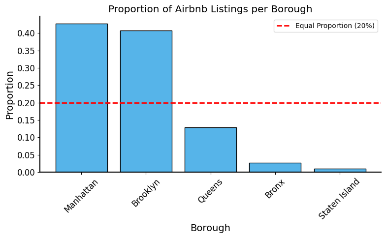
For example, we might assume that the all Airbnb listings in New York City are equally likely to be in any one of the five boroughs. (So the probability of a listing being in Manhattan is 1/5, the probability of it being in Brooklyn is 1/5, etc.)
Then we can look at the actual sample of listings and see if it matches our assumption:
Code
# number of listings per boroughborough_counts = airbnb['borough'].value_counts().rename_axis('borough').reset_index(name='count')borough_counts['borough'] = borough_counts['borough'].str.title() # capitalize# normalize the counts to proportionsborough_counts['proportion'] = borough_counts['count'] / borough_counts['count'].sum()plt.figure(figsize=(8, 5))plt.bar(borough_counts['borough'], borough_counts['proportion'])plt.axhline(y=1/5, color='r', linestyle='--', label='Equal Proportion (20%)')plt.title('Proportion of Airbnb Listings per Borough')plt.xlabel('Borough', fontsize=14)plt.ylabel('Proportion', fontsize=14)plt.xticks(rotation=45)plt.legend()plt.tight_layout()plt.show()
The inference question we want to ask is roughly:
“If we assume that all boroughs are equally likely to produce each listing, how likely is it that we would see the distribution of listings that we actually observe?”
Notice that this is a question about the probability of the sample, given a certain model of the DGP. In our Airbnb example above, it intuitively seems unlikely that we would see so many more listings in Manhattan and Brooklyn than in the other boroughs if all boroughs were equally likely to produce listings.
What should we do now? Now that we realize our sample is very unlikely under our model, then perhaps we should reconsider our model. After all, the model is just a “guess” about the DGP, while the sample is real data that we have observed.
Unlikely data or unlikely model?
There are two main culprits when we see a sample that is unlikely under our model:
The sample! Think of this as “luck of the draw”. This is only really a risk if your sample is small or systematically biased in some way. Usually if you collect enough data, the sample will start to look more like the population. If you flip a coin 5 times, you might get all tails (there’s actually a 3% chance of this happening); if you flip a coin 100 times, there’s virtually no chance that you’ll get all tails (less than 10-30 chance).
The model! This means that our assumptions about the DGP are incorrect or incomplete. This is a more serious problem, and it won’t go away just by collecting more data.
Statistical inference is basically just a bunch of mathematical machinery and techniques that help us to quantify this guesswork precisely and make it rigorous.
Don’t try this at home!
We just said that statistical inference makes guesswork rigorous, but this is not the whole story.
We will always do a much better job of inference if was have a good understanding of the DGP and the context of the data. This requires domain knowledge and subject matter expertise. In the Airbnb example, you would want to know something about the five boroughs of New York City before starting your analysis. Assuming that all boroughs are equally likely to produce listings is a pretty bad assumption (Manhattan sees vastly more tourism than the other boroughs, and Brooklyn and Queens have by far the most residents according to recent census data).
Statistical inference is a powerful tool, but it is not a substitute for understanding the data and the context in which it was collected. Modeling might be guesswork, but it is best if it is informed guesswork.
Prediction
Prediction is the process of using a model to make predictions about unseen (or future) data.
Back to the Airbnb data, we might want to predict which borough a new listing belongs to based on its features (e.g., listing type, review ratings, price, etc.).
To that end we will fit a predictive model to the data. We won’t go into the details of the model we use here, but the basic idea is that we assume the features of the listing (e.g., price) is related to the probability of it being in a certain borough (perhaps more expensive listings are more likely to be in Manhattan, for example).
Fitting a model
Models generally have parameters, which are adjustable values that affect the model’s behavior. Think of them like “knobs” you can turn to tune the model to do what you want, like adjusting the volume or the bass/treble on a speaker.
The model for a coin flip, for example, has a single parameter: the probability of landing on heads. If you turn the knob to 0.5, you get a fair coin; if you turn it to 1.0, you get a coin that always lands on heads; if you turn it to 0.0, you get a coin that always lands on tails.
Fitting a model means adjusting the parameters of the model so that it best matches the data. This is usually done by minimizing some kind of error function, which provides a measure of how well the model fits the data.
Code
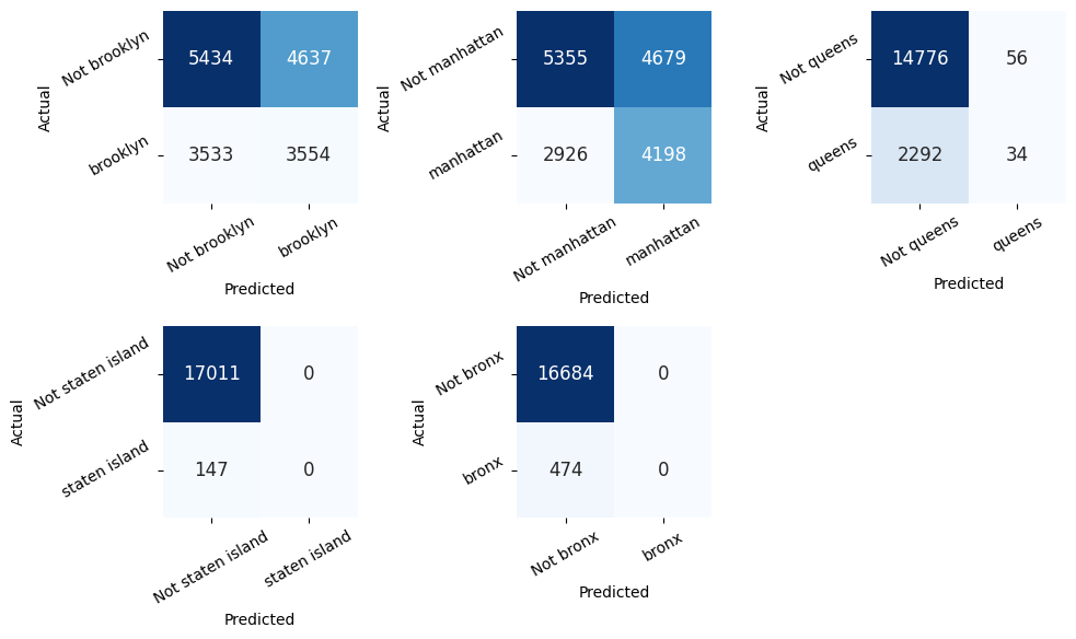
from sklearn.linear_model import LinearRegression, LogisticRegressionfrom sklearn.model_selection import train_test_splitfrom sklearn.metrics import multilabel_confusion_matriximport seaborn as sns# prepare the data for linear regressionfeature_columns = ["price", "room_type", "minimum_nights", "number_of_reviews", "reviews_per_month", "review_rate_number"]airbnb_clean = airbnb.dropna(subset=feature_columns + ["borough"])X = airbnb_clean[feature_columns]# convert categorical variables to lowercaseX.loc[:, "room_type"] = X["room_type"].str.lower()y = airbnb_clean["borough"].values.reshape(-1)# convert categorical variables to dummy variablesX = pd.get_dummies(X, columns=["room_type"], drop_first=True)X["rating_interaction"] = X["reviews_per_month"] * X["review_rate_number"]# split the data into training and test setsX_train, X_test, y_train, y_test = train_test_split(X, y, test_size=0.2, random_state=56)# fit the logistic regression modelmodel = LogisticRegression(max_iter=1000, solver="newton-cholesky")model.fit(X_train, y_train)# make predictions on the test sety_pred = model.predict(X_test)# calculate the prediction accuracyaccuracy = np.mean(y_pred == y_test)print(f"{40*'='}")print(f'Prediction Accuracy: {accuracy:.2%}')print(f"{40*'='}")# calculate the confusion matrixconfusion_matrix = multilabel_confusion_matrix(y_test, y_pred, labels=airbnb['borough'].unique())# confusion_matrix = [confusion_matrix[i].T for i in range(len(confusion_matrix))] fig, ax = plt.subplots(2, 3, figsize=(10, 6))ax = ax.flatten()ax[-1].axis('off') # turn off the last subplot since we have only 5 boroughs# plot the confusion matrix for each boroughfor i, borough inenumerate(airbnb['borough'].unique()): sns.heatmap(confusion_matrix[i], annot=True, fmt='d', cmap='Blues', ax=ax[i], cbar=False) ax[i].set_xlabel('Predicted', fontsize=10) ax[i].set_ylabel('Actual', fontsize=10) ax[i].set_xticklabels(['Not '+ borough, borough], rotation=30, fontsize=10) ax[i].set_yticklabels(['Not '+ borough, borough], rotation=30, fontsize=10)plt.tight_layout()_ = plt.show()
Ok, so the model is around 45% accurate at predicting the borough of a listing.
What is a “good” prediction rate?
For discussion / reflection: What is a “good” prediction rate or accuracy? Is 45% good? What about 60%? 80%? How would you tell?
Later in the course, we will talk about how to evaluate models and prediction accuracy more rigorously. For now, just keep in mind that there is no one-size-fits-all answer to this question. It depends on factors like what you want to do with the model or how good simple alternatives might be. For example, you want self-driving cars to be nearly 100% accurate because the cost of a mistake is so high. Perhaps a general manager drafting prospective players for a sports team would be satisfied with 60% accuracy, since they only need to be right about some players to make a big difference in the team’s performance.
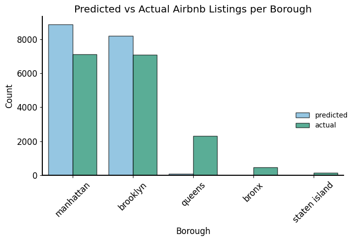
Now let’s take a look at the distribution of the model’s predictions.
Code
# plot the counts of predicted listings per borough side by side with the actual countsimport seaborn as snsplot_df = pd.DataFrame({'predicted': pd.Series(y_pred.flatten()),'actual': pd.Series(y_test.flatten())})plot_df = plot_df.melt(var_name='type', value_name='borough')fig, ax = plt.subplots(figsize=(10, 6))sns.countplot(x='borough', hue='type', data=plot_df, ax=ax, alpha=0.7)sns.move_legend(ax, loc="center right", title=None)plt.title('Predicted vs Actual Airbnb Listings per Borough')plt.xlabel('Borough')plt.ylabel('Count')plt.xticks(rotation=45)plt.tight_layout()plt.show()
It looks like the model is a bit crude (it predicts no listings in the Bronx or Staten Island), but it does at least capture the general trend that listings are more likely to be in Manhattan and Brooklyn than in the other boroughs.
Prediction and inference can interact
Prediction and inference are closely related, and they can often be done simultaneously.
The guiding logic is that a model that makes good predictions is probably doing a good job of capturing the underlying DGP.
Summary
In this introductory lecture we talked about the 3 objectives of data analysis: description, inference, and prediction. Hopefully you now have a better understanding of what statistics is supposed to help you do with data. Of course, we haven’t actually gone into any of the details of how to do anything. Don’t worry, we’ll get there!
Next up, we’ll cover some of the basic programming concepts that are important for data science. After that we will learn some foundational concepts in probability that will help us think about data and models more rigorously. From there, the sky is the limit! We’ll cover a wide range of topics, including statistical inference, uncertainty quantification, machine learning, and more.
Since we haven’t learned any programming or statistics yet, we won’t have any real exercises for this lecture. There’s just a quick Assignment 0 to make sure you are set up to run Python code for future assignments.